Lorem ipsum dolor sit amet, consectetur adipiscing elit, sed do eiusmod tempor incididunt ut labore et dolore magna aliqua. Ut enim ad minim veniam, quis nostrud exercitation ullamco laboris nisi ut aliquip ex ea commodo consequat. Duis aute irure dolor in reprehenderit in voluptate velit esse cillum dolore eu fugiat nulla pariatur.
Migrating from Rev.ai to Gladia: what global teams should know
TL;DR: At 10,000 hours of audio per month, Rev.ai's per-hour billing compounds quickly once you add diarization, translation, and sentiment as separate line items. Language coverage gaps surface silently in production when non-English or accented audio degrades without returning an obvious error. This guide gives you the exact API payload mappings, WebSocket transition logic, and a TCO model at realistic scale to make a defensible evaluation of switching. If you decide to migrate, our all-inclusive per-hour pricing bundles every audio intelligence feature at the base rate, and most teams complete the endpoint transition and initial production validation in under 24 hours.
Switching your speech-to-text provider: A migration checklist for note-takers and contact center platforms
TL;DR: Switching your speech-to-text provider is a structural risk only if you skip the pre-migration audit. The real danger is not the cutover itself but continuing to run infrastructure that corrupts CRM entries, breaks LLM summaries, and inflates your per-hour cost with add-on fees you never modeled at scale. The four-stage phased cutover in this guide is designed to reach 100% production traffic without user-visible downtime, the same structural approach that let Aircall cut processing time by 95% and scale to over one million calls per week after adopting Gladia.
How decision intelligence improves customer service consistency in contact centers
TL;DR: Contact centers fail to deliver consistent service when routing infrastructure runs on static rules engines that cannot handle the complexity of real human conversation. Modern speech-to-text infrastructure addresses this by processing raw audio and feeding structured outputs to your CRM, using machine learning to analyze intent, sentiment, and speaker characteristics. Transcription accuracy sets the ceiling for every downstream action: a wrong word silently corrupts a CRM entry, a missed intent misfires a routing decision, and a misread sentiment score delays escalation. This playbook covers how to build and deploy that architecture without blowing your latency budget or your unit economics.
One of the major obstacles for speech-to-text AI has been identifying individual speakers in a multi-speaker audio stream before transcribing the speech. This is where speaker separation, also known as diarization, comes into play.
Speech recognition systems have improved dramatically in the last decade. Large neural automatic speech recognition (ASR) models can now achieve very low word error rates (WER) on many benchmarks. But transcription accuracy alone does not make speech data usable.
In real conversations, multiple people speak. They interrupt each other. They pause, overlap, and switch turns quickly. A transcript that captures the words but loses who said them is often insufficient for downstream applications. This is where speaker diarization becomes critical. Diarization answers a simple but technically difficult question:
Who spoke when in the recording?
Without diarization, transcripts of meetings, interviews, podcasts, or customer calls become flat text streams. Once speaker attribution is lost, downstream systems such as summarization models, analytics pipelines, or compliance checks lose important context. For engineers building voice applications, diarization is therefore not a cosmetic feature. It is a structural component of production speech pipelines.
TL;DR
While speech-to-text converts audio into words, diarization assigns those words to the correct speakers, determining who speaks when.
Modern diarization systems combine neural segmentation models, speaker embeddings, and clustering algorithms to group speech segments by speaker identity.
Performance is measured using diarization error rate (DER).
Benchmarks like the DIHARD challenge datasets are widely used because they reflect realistic multi-speaker environments.
Gladia supports speaker diarization for asynchronous (batch) transcription, where the full recording is analyzed before generating the final transcript.
What speaker diarization means in practice
Speaker diarization is the process of segmenting an audio recording into time intervals associated with individual speakers. A diarization system receives an audio signal and produces a timeline like this:
0:00–0:05  Speaker A
0:05–0:07  Speaker B
0:07–0:10  Speaker A
These speaker segments are then aligned with the transcription output to produce a structured transcript.
So the typical diarized transcript might look like:
Speaker 1: Let’s review the metrics from last quarter.
Speaker 2: Sure. Revenue increased by twelve percent.
Speaker 1: That’s better than expected.
The goal is not necessarily to identify the actual identity of the speakers. Most diarization systems simply assign anonymous labels such as Speaker 1, Speaker 2, and so on. The objective is consistent speaker attribution across the conversation.
Why diarization matters for real voice applications
Many modern voice systems rely on speaker structure to function correctly. Consider a few common production scenarios.
Meeting assistants and note-takers: Meeting transcription systems rely on diarization to produce speaker-based transcripts and summaries. If speaker attribution is wrong, summaries can attribute decisions or action items to the wrong participant. This quickly erodes trust in meeting tools, especially when action items are assigned to the wrong person.
Conversation analytics: Customer support platforms often measure talk-time ratios between agents and customers. Without diarization, these metrics cannot be computed reliably. It also becomes difficult to detect interruptions, long monologues, or customer frustration patterns.
Voice agents analyzing conversations: These rely on diarized transcripts to understand dialogue structure. Without speaker separation, the agent cannot reliably determine who asked a question, who responded, or how the conversation evolved.
Podcast and media indexing: Media archives use diarization to identify distinct speaker segments, enabling searchable speaker timelines and content indexing. This allows listeners to jump directly to a specific guest or speaker within long recordings.
In all these systems, diarization errors propagate downstream. A transcript with perfect WER but incorrect speaker attribution can still break the application logic built on top of it.
How diarization works in speech pipelines
Modern diarization systems typically follow a multi-stage architecture. While implementations differ, most pipelines include three core components:
speech segmentation
speaker representation (embeddings)
clustering
This architecture has become standard in neural diarization systems.
Speech segmentation
The first step is identifying when speech occurs in the recording. This stage often relies on voice activity detection (VAD) to remove silence and background noise. Once speech segments are detected, a segmentation model determines where speaker changes occur. The output of this stage is a timeline of short audio streams where a speaker is assumed to remain constant. At this point, the system does not yet know which speaker produced each segment.
Speaker embeddings
Next, the system generates speaker embeddings for each segment.
A speaker embedding is a vector representation capturing distinctive characteristics of a voice, such as pitch, spectral patterns, and speaking style. Speaker embeddings are typically learned using deep neural networks trained for speaker verification tasks, where the objective is to map recordings from the same speaker close together in embedding space while separating different speakers. Segments produced by the same speaker tend to generate embeddings that are close to each other in the embedding space.
Embedding models are typically trained using large datasets of labeled speaker audio. These embeddings allow the system to compare different segments and determine whether they likely originate from the same speaker.
Clustering
Once embeddings are computed, the system groups segments into speaker clusters. Clustering algorithms analyze similarity between embeddings and assign segments to speaker groups. Each cluster represents a single global speaker within the recording. After clustering, the diarization timeline can be reconstructed with consistent speaker labels.
Common diarization failure modes
Despite major advances in neural speech processing, diarization remains difficult on real-world audio data. Several factors strongly affect performance:
Overlapping speech: When two speakers talk simultaneously, segmentation models struggle to assign segments cleanly. Overlapping speech is one of the largest contributors to diarization error.
Short speaker turns: Rapid back-and-forth conversations create extremely short segments that are harder to cluster reliably.
Background noise: Environmental noise can distort speaker features and degrade embedding quality.
Domain mismatch: Models trained on broadcast speech may perform poorly on conversational audio files or field recordings.
These challenges explain why diarization accuracy is still an active research area.
Measuring diarization accuracy with DER
Diarization systems are evaluated using diarization error rate (DER). DER combines three types of errors:
Missed speech: speech segments incorrectly labeled as silence
False alarms: non-speech segments labeled as speech
Speaker confusion: segments attributed to the wrong speaker
The final DER score represents the percentage of time where the diarization output differs from the ground truth. Lower DER indicates better diarization performance.
Evaluating diarization with benchmark datasets
Realistic evaluation requires datasets containing complex multi-speaker recordings. One of the most widely used evaluation frameworks is the DIHARD Speech Diarization Challenge. These datasets include recordings from diverse domains such as meetings, broadcasts, web videos, and field recordings.
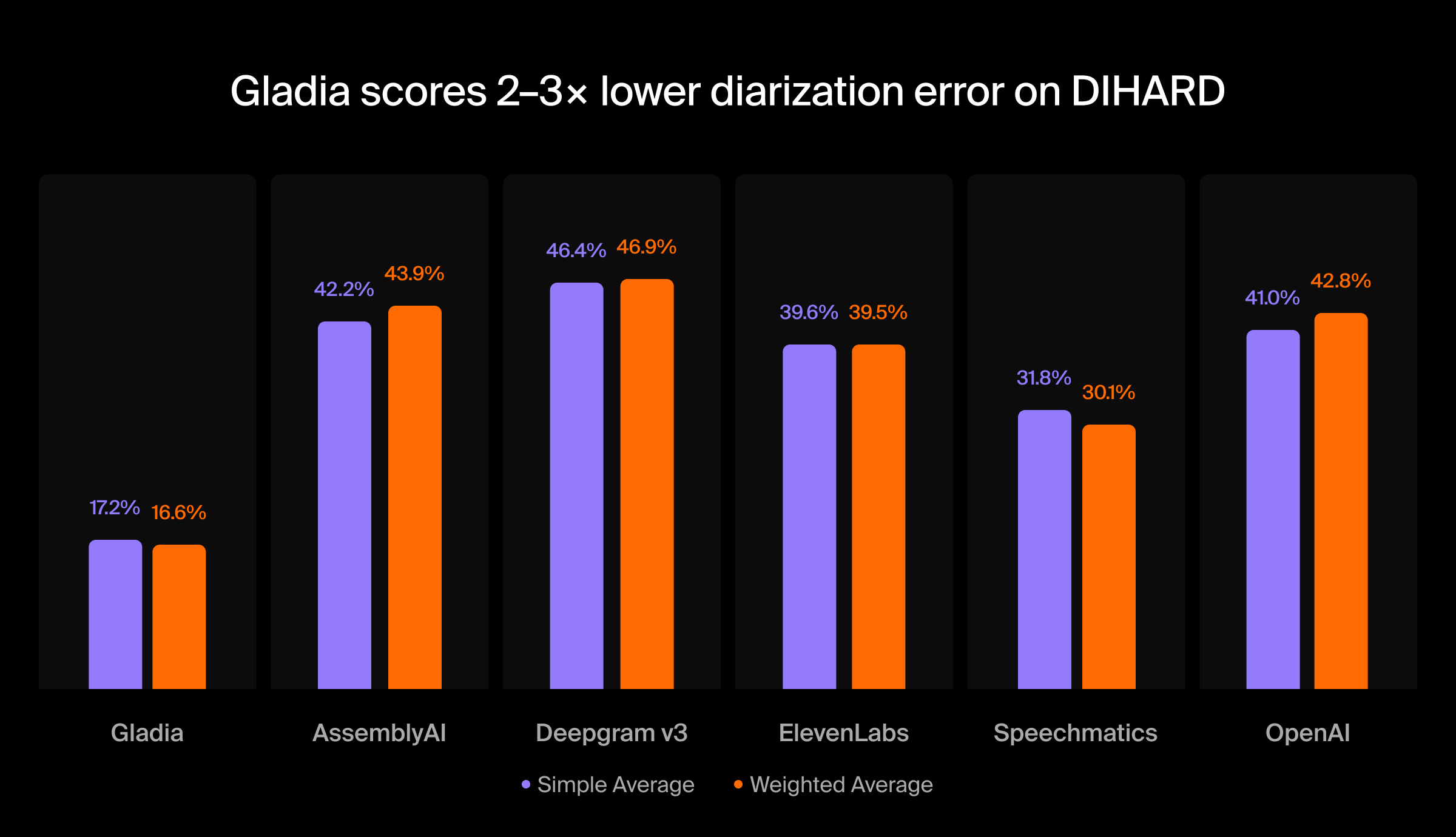
Gladia’s latest benchmarks show diarization results across multiple DIHARD scenarios, including broadcast audio, meeting recordings, restaurant environments, and clinical conversations. These environments are intentionally difficult. They include background noise, overlapping speech, and conversational dynamics that resemble real production audio.
According to the benchmark results, diarization error rates vary significantly depending on the dataset and environment. For example, different systems show substantially higher DER on challenging scenarios such as web video or restaurant audio compared to structured recordings like broadcast speech.
Across the DIHARD datasets included in the benchmarks, Gladia’s diarization system achieves a weighted average DER of 16.6%, a substantially higher DER values for several commercial speech APIs. Put differently, the results show roughly 2-3x fewer diarization errors than competing systems in many scenarios.
These results come from significant work on Gladia’s proprietary diarization stack, leveraging pyannoteAI’s state-of-the-art Precision-2 diarization models. Pyannote-based diarization systems are widely used in both academic research and production speech pipelines due to their modular architecture and strong benchmark performance.
The key takeaway is that diarization performance is highly dependent on audio conditions. Models that appear strong on clean datasets may degrade substantially when exposed to real conversational audio. Evaluating systems across diverse domains is therefore essential when selecting a diarization pipeline for production voice applications.
How diarization fits into production speech architectures
In production voice systems, diarization typically runs as a stage within the broader speech processing pipeline. A simplified architecture looks like this:
Audio ingestion → preprocessing / VAD → speaker diarization → speech recognition → alignment and transcript formatting → downstream AI processing.
There are two main reasons diarization is often performed before final transcript formatting: First, diarization models rely on raw acoustic signals. Running diarization on the audio rather than the transcript avoids losing speaker cues embedded in the waveform. Second, diarization allows transcripts to be structured correctly before they are consumed by downstream systems such as summarization models, analytics pipelines, or conversational AI agents.
In batch pipelines, the diarization model can analyze the entire recording at once, allowing clustering algorithms to see the full conversation context. This global context improves speaker consistency across the transcript.
Diarization in Gladia’s speech pipeline
Gladia integrates diarization into its asynchronous transcription pipeline, where the entire audio recording is processed before generating the final structured transcript. The diarization system relies on pyannote-based models, including the “precision-2” diarization model, which is publicly benchmarked on the DIHARD datasets. Because the full recording is available during processing, the system can:
Compute speaker embeddings across the entire conversation
Cluster segments using global context
Align speaker segments with the final transcription output
This batch processing architecture is particularly well-suited for recordings such as meetings, podcasts, interviews, and recorded customer calls.
At the moment, diarization is supported only for asynchronous transcription workflows, where the system can analyze the full audio recording before producing the final transcript.
How to perform speaker diarization in practice
In Gladia’s transcription API, diarization can be enabled directly in the transcription request. For pre-recorded audio, this is done by adding the diarization parameter:
When diarization is enabled, the transcription response includes a speaker field for each utterance. Speakers are indexed in the order they appear in the recording.
In some scenarios, diarization accuracy can improve if the system receives hints about the expected number of speakers in the conversation. More about that in our documentation.
FAQs
How accurate is speaker diarization?
Accuracy varies depending on the recording conditions. Clean recordings with clear speaker turns may achieve low DER, while noisy environments with overlapping speech can significantly increase diarization errors.
What affects DER the most?
The largest contributors to diarization errors are overlapping speech, rapid speaker turn-taking, background noise, and domain mismatch between training data and real-world audio.
Can diarization work in real time?
Real-time diarization is technically possible but significantly more challenging. Many systems perform more reliably in batch pipelines where the entire recording can be analyzed before clustering speakers.
How does diarization interact with transcription models?
Diarization determines the speaker timeline, while ASR models convert speech into text. The two outputs are combined to produce transcripts where each segment is attributed to the correct speaker.
Why does diarization break on overlapping speech?
Most diarization models assume that a single speaker dominates a segment of audio. When multiple speakers talk simultaneously, the acoustic features of their voices mix, making segmentation and clustering significantly harder. Overlapping speech remains one of the hardest problems in speaker diarization research and is a major focus of the DIHARD challenge datasets.
Key terminology
Speaker diarization: The task of determining which speaker produced each segment of speech in a multi-speaker audio recording.
Diarization error rate (DER): The standard evaluation metric for diarization systems. It measures the percentage of time where the predicted speaker timeline differs from the ground truth.
Speaker attribution: The process of assigning spoken segments in a transcript to the correct speaker.
Segmentation: The step where an audio recording is divided into smaller time segments where speaker identity is assumed to be constant.
Speaker embeddings: Vector representations that capture distinctive characteristics of a speaker’s voice and allow similarity comparisons between speech segments.
Clustering: The process of grouping speaker embeddings to determine which segments belong to the same speaker.
Overlapping speech: Audio segments where multiple speakers talk simultaneously. These segments are difficult for diarization systems and often increase DER.
Contact us
Your request has been registered
A problem occurred while submitting the form.
Read more
Speech-To-Text
Migrating from Rev.ai to Gladia: what global teams should know
Speech-To-Text
Switching your speech-to-text provider: a migration checklist for note-takers and CCaaS
Speech-To-Text
How decision intelligence improves customer service consistency in contact centers
From audio to knowledge
Subscribe to receive latest news, product updates and curated AI content.
Thank you! Your submission has been received!
Oops! Something went wrong while submitting the form.